TOPIC: GIS

The National Oceanic and Atmospheric Administration (NOAA) provides free access to their Data Access Viewer (DAV). The DAV allows users to search for and download various data types for the coastal U.S. and its territories. The data types available are elevation, imagery, and land cover data. This data can be useful on all phases of a design project, so let’s explore how to access LiDAR data for use in Autodesk applications that support point clouds.

Data Access Viewer (DAV)

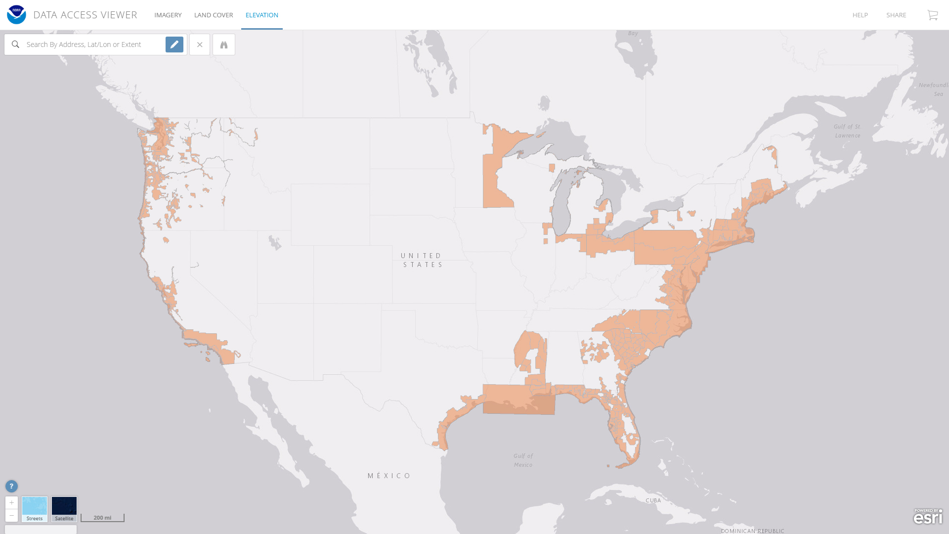
NOAA’s Data Access Viewer (DAV) can be accessed via this link (https://coast.noaa.gov/dataviewer/#/) and can be used to access elevation, land cover, and imagery datasets for the coastal regions of the United States.

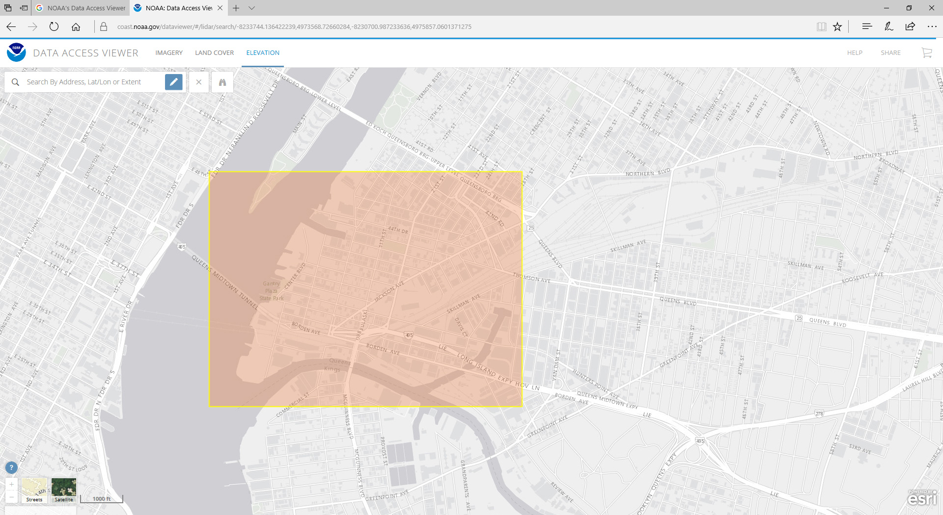
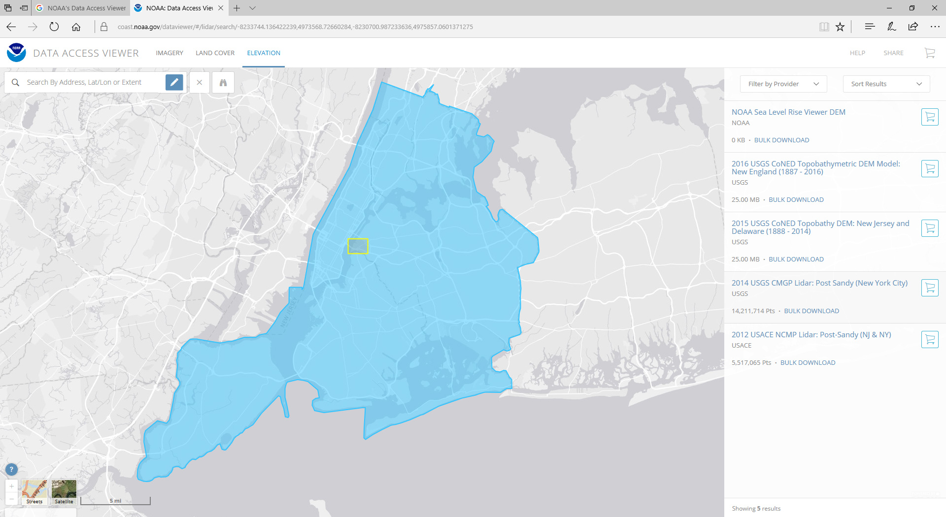
After selecting Elevation, zoom into or draw your area of interest (AOI). Alternatively, enter in an address or the coordinates of your project area. You can then see the available data for that region or range. I’ve drawn a region around Long Island City, NY for this example. For that AOI there are three DEM files (digital elevation models) and two LiDAR files are available.

Finding LIDAR data

I’m interested in the latest LIDAR scan from the USGS and so I have one of two additional choices. I can use the bulk download feature to download the various tiles that make up my AOI. Alternatively, I can add my request to the cart and let NOAA’s servers process the request to only provide the points bound by my AOI. I will choose the latter which allows me to make additional changes to how I want to receive the data.

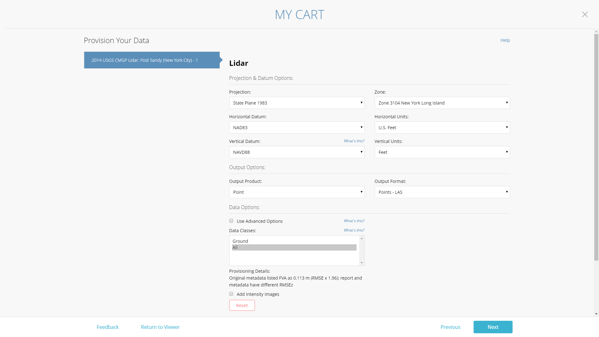
I want point cloud information, so I need to change the OUTPUT PRODUCT from Raster to Point. Additionally, I will verify the output format is an LAS file, a format that can be imported into Autodesk Recap. Lastly, I will verify that Data Classes include all points, not just the ground points. To wrap up, enter an email address to allow NOAA’s servers to contact you once the job is ready for download. Click the image on left to see these settings.

Importing the LAS file

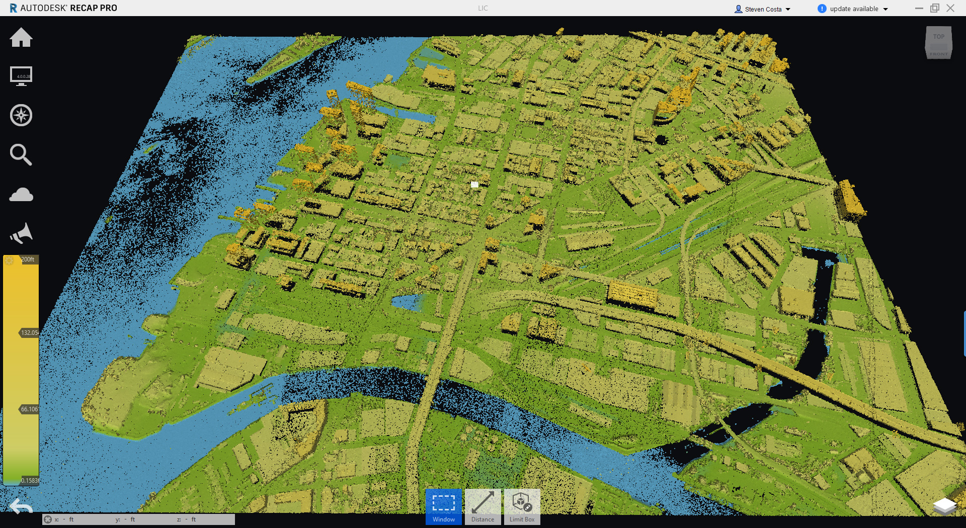
The processing time for this job example took about 5 minutes to generate. Once you have received and downloaded your LiDAR scan you will want to import the LAS file(s) into AutoCAD ReCap. Processing the LiDAR scan in Recap allows you to use this scan in Autodesk products such as Civil 3D, Revit, Navisworks, Infraworks, and 3ds Max.

To begin, create and name a new Recap project by choosing a project name directory to store the project. Next, using Windows Explorer, browse to the LAS file(s) you extracted and drag-and-drop them onto Recap.

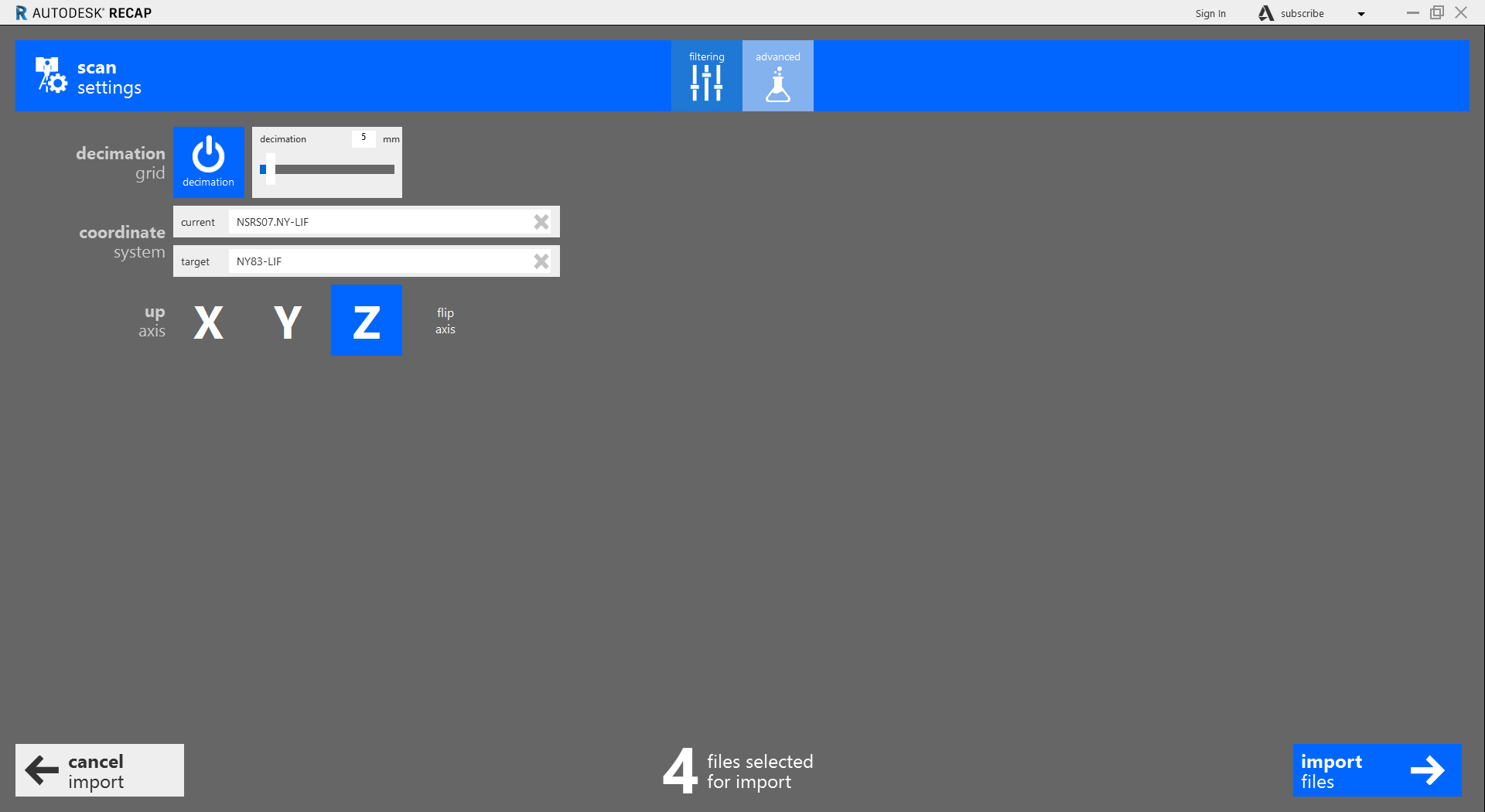
Dragging and dropping these files onto the target icon in ReCap will take you to a screen where you can change the Scan Settings.

Click on Advanced Settings. It’s important to note it is only at this point of the importing process that you can transform the LiDAR scan from its original coordinate system to your desired coordinate system.

Since the site is in Queens, NY, I will be using the NY State Plane Coordinate System NY83-LIF. This datum, (North American Datum 1983, Long Island Zone, US Survey Feet) is used for the 5 boroughs of NYC and Long Island. After setting the coordinate system, select, Import files, then index scans, and when the files are indexed, click Launch Project.

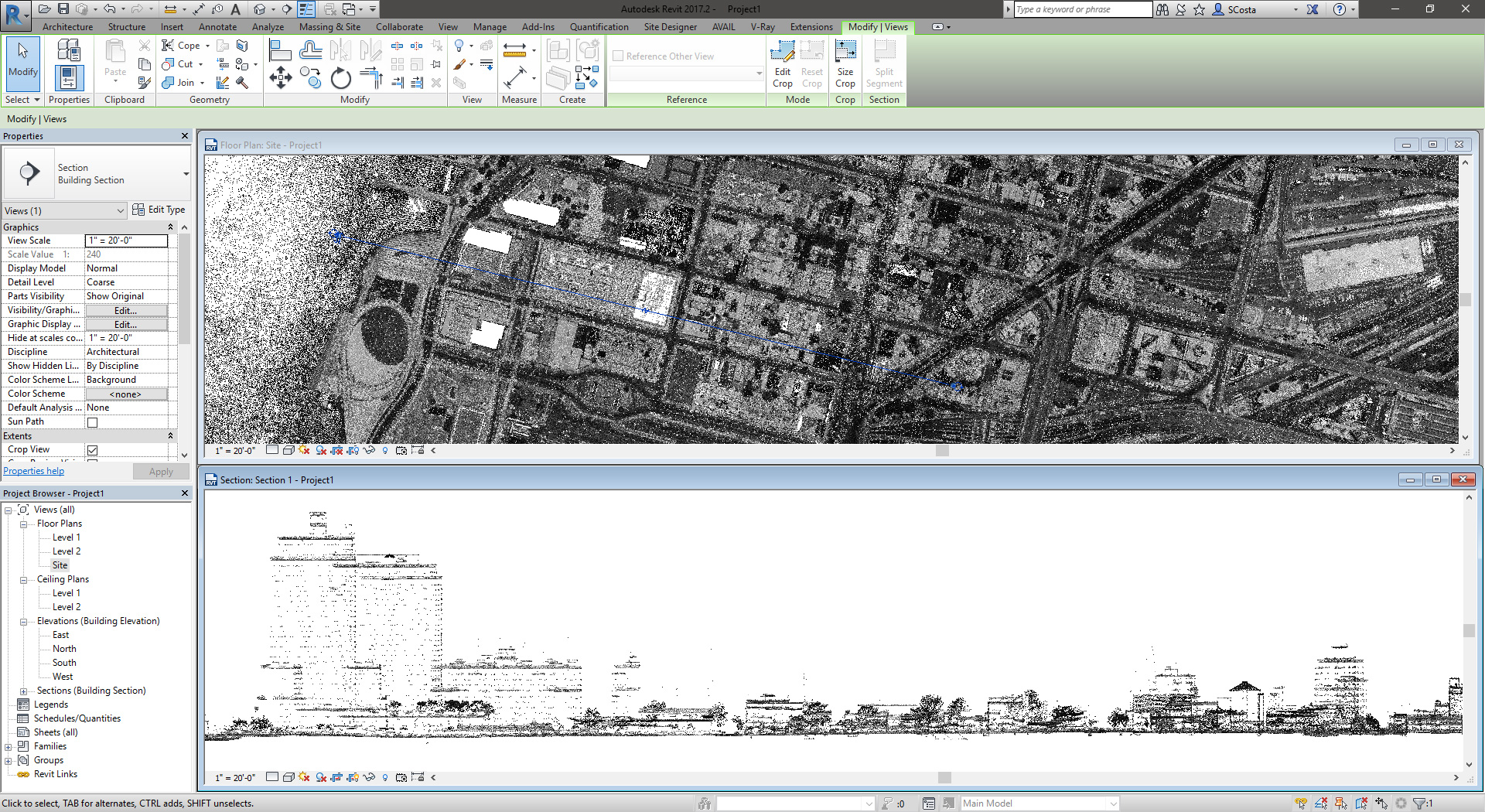
Once opened, save the project and you will have an RCP file you can link into products like Civil 3D, Revit, and Infraworks.

A recent question on the Civil 3D Forums had me wondering whether it was possible to display ponding water on a Civil 3D surface. I was certain there wasn’t a push-a-button-get-an-answer solution, but I decided to see if I could get the job done using a combination of Civil 3D tools.

To understand where ponding could occur on this surface, one would need to analyze the surface and identify which regions of the surface contain depressions where water could collect. Depending on how many local low points there may be on the surface, it’s likely that any analysis would need to be iterative and require a certain amount of user input.

While the solution I present below works for some Civil 3D surfaces, the actual question posted on the Civil 3D Forums asked about a large and complex DEM (digital elevation model). With that in mind, I will be making additional suggestions for complex analysis using another application better suited for the task in a separate blog post.

EXTRACT A DEPRESSION AREA

I’ll begin with a Civil 3D surface, one readily available with every installation of the product. The simplest way to do an analysis of the drainage areas of a surface is to run a watershed analysis. When running the analysis, I am only going to be focusing on the depressions on that surface. Once again, depending on your surface geometry, you may get one or more depressions, or you may get none. In the surface I am working with, there are six distinct depression areas, however I will be focusing in on the largest of the six for the purposes of this blog.

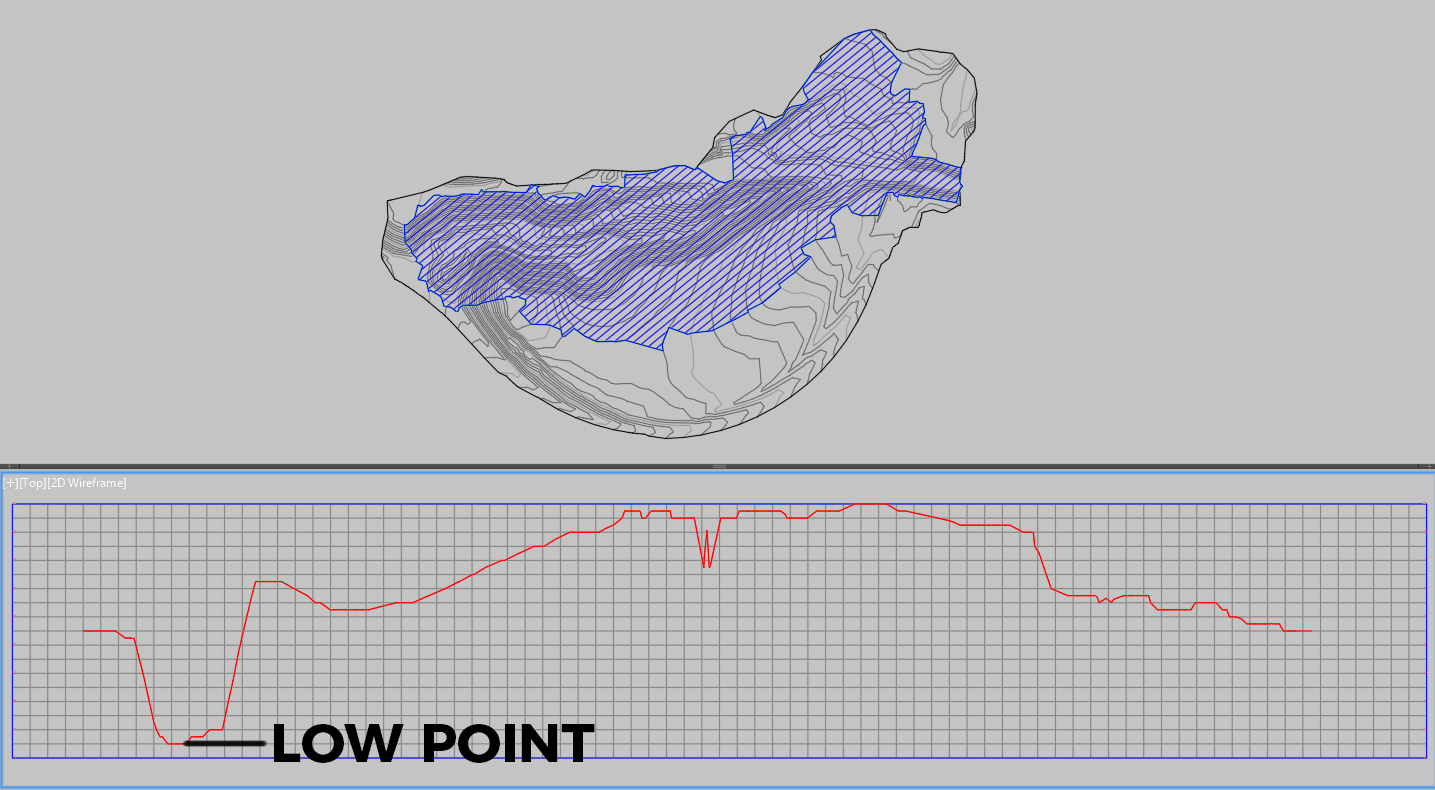
Once I have identified the depression I want to work with, the next step is to determine the lowest point on the edge of that depression since it will be the “spill over” point, that is, the point at which water will drain into the adjacent area on the surface. Again, there are several ways to accomplish this task, but I found the quickest non-lisp related way to find the lowest elevation point is to:

1. Select the surface and use the Extract from Surface tool
2. Next, select only Watersheds → Select Manually and choose the depression boundary, then press OK
3. In model space, select the extracted 3D Polyline, right-click and choose Quick Profile
4. Choose a basic Profile View style, select OK, and then select a point to place the Profile View
5. Select the existing ground Profile, right-click and choose Profile Properties
6. Make the Profile Data tab active and make note of the minimum elevation for the profile

IDENTIFY THE SPILL-OVER ELEVATION

Once you have the minimum elevation of that boundary, you can then use that same extracted boundary edge to temporarily create an outer boundary for the surface you are analyzing. Doing so, and then examining the surface properties, would reveal the minimum elevation of the surface within that depression. This will give you the delta between the low point and the spill-over point. Alternatively, you could create a “zero elevation” surface and use the Minimum Distance Between Surfaces to find the low point on the EG surface.

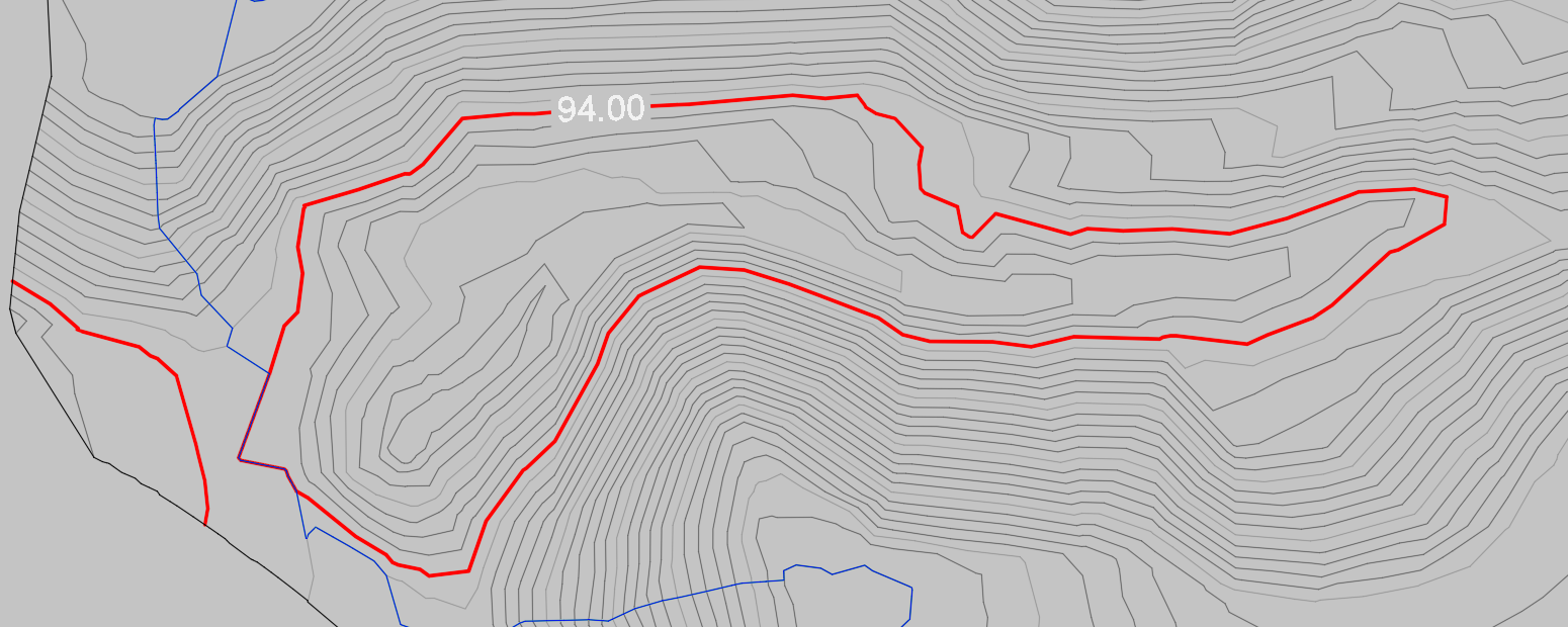
Using the spill-over elevation, you can now create a user contour set to that elevation and style it for easy visibility. To do so:

1. Select the surface, right-click and choose Surface Properties
2. Select the Analysis tab and choose User-Defined Contours from the Analysis type drop-down menu
3. Add one range and select Run Analysis
4. Set the elevation of that user-defined contour to the spill-over value and press OK.

STYLE THE USER CONTOUR

To see that contour on your surface you will need enable User Contours on the surfaces current style . We will then extract that contour as a polyline to use for our POND surface. To do so, follow these steps which are similar to the ones above:

1. Select the surface and use the Extract from Surface tool
2. Select only User Contours → Select Manually and choose the user contour within the depression boundary you are analyzing. If only one contour exists, Civil 3D will default to Select All.

I had to do some minor clean-up of the line-work in my example as there were some duplicate lines, but in the end, I now have a boundary representing my ponding limits. The last step is to create a surface called POND from the extracted polyline. You should use that polyline to define both the breakline elevations and the outer boundary of the surface.

VISUALIZE YOUR PONDING AREA

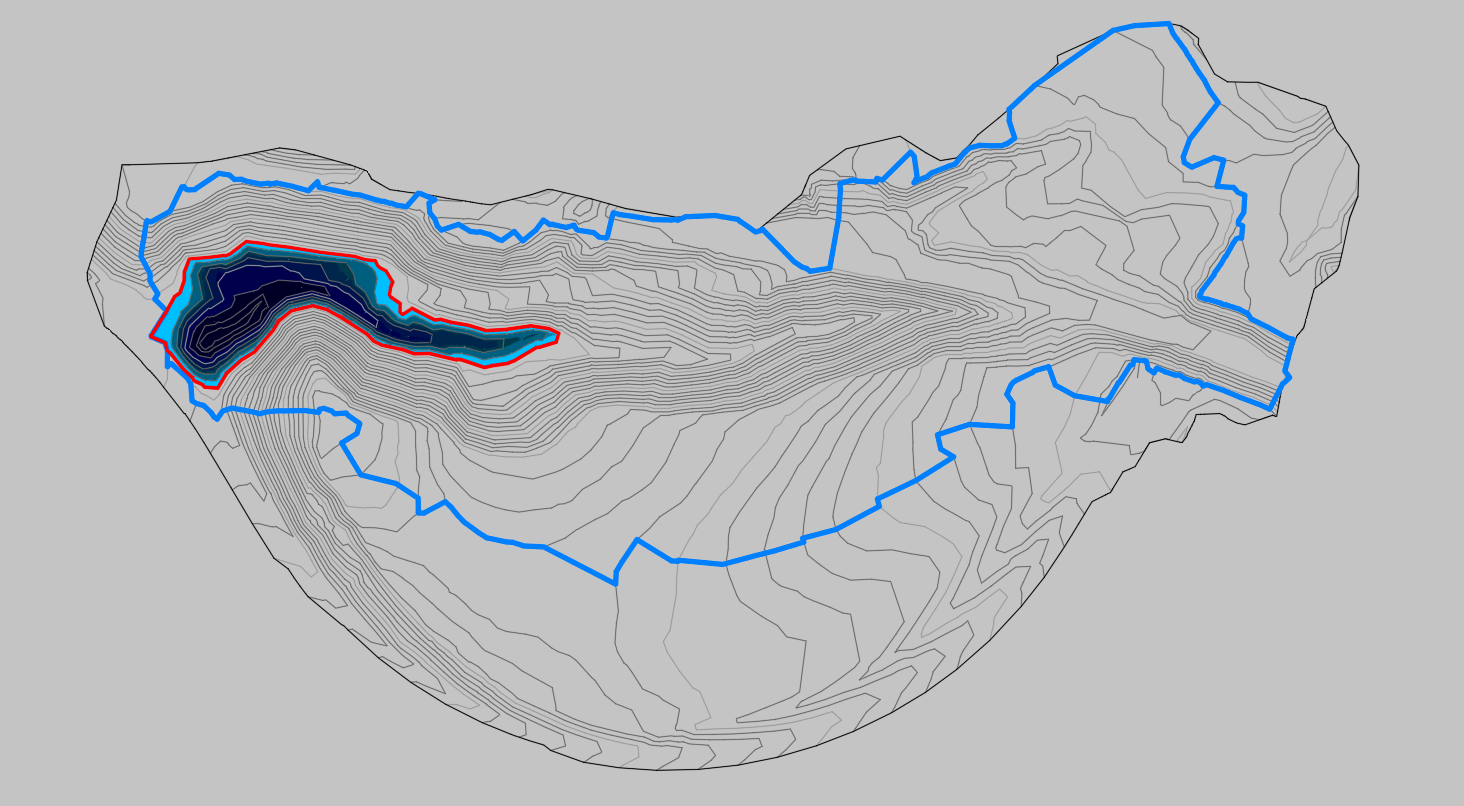
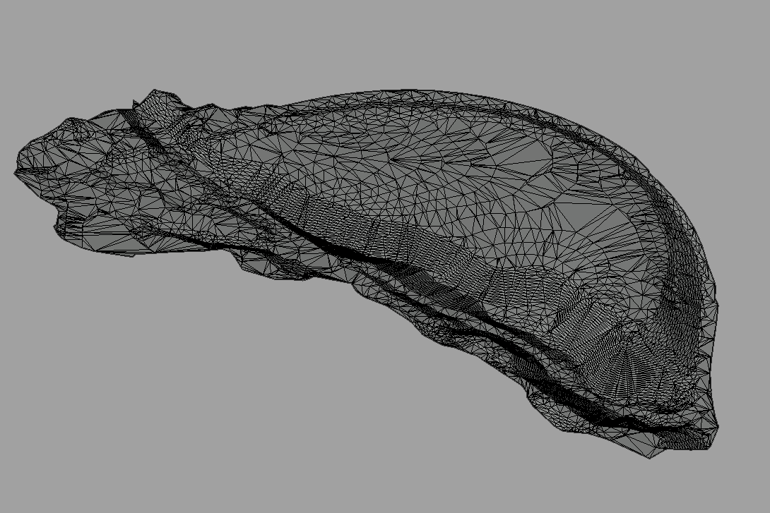
You can now use that surface to do any type of visualization that you would need. As an example, create a volume surface and run an elevation analysis to determine the depth/distribution of the ponding. See the image below for an example.